For the final assignment, I decided to run an Anova using the DIET_EXERCISE dataset, for the sole reason that it is the onlly data set with a variable that can be used as a moderator that has limited number of values (categorical).

The code I run can be seen below, and you can copy and paste it on SAS Code tab to make sure it works.

---

/*
*
* Task code generated by SAS Studio 3.5
*
* Generated on ’24/1/17 – 4:35 μ.μ.’
* Generated by ‘epanagiotopoulo0’
* Generated on server ‘ODAWS02.ODA.SAS.COM’
* Generated on SAS platform ‘Linux LIN X64 3.10.0-514.2.2.el7.x86_64’
* Generated on SAS version ‘9.04.01M3P06242015’
* Generated on browser ‘Mozilla/5.0 (Windows NT 10.0; WOW64; rv:50.0) Gecko/20100101 Firefox/50.0’
* Generated on web client ‘https://odamid.oda.sas.com/SASStudio/main?locale=el_GR&zone=GMT%252B02%253A00&https%3A%2F%2Fodamid.oda.sas.com%2FSASStudio%2F=’
*
*/

ods noproctitle;
ods graphics / imagemap=on;

proc glm data=_TEMP0.DIET_EXERCISE;
class Exercise Diet;
model WeightLoss=Exercise Diet Exercise*Diet / ss1 ss3;
lsmeans Exercise*Diet / adjust=tukey pdiff=all alpha=0.05 cl;
quit;

---

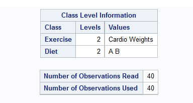
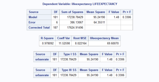
You can see that all of the observations have been used for this analysis.

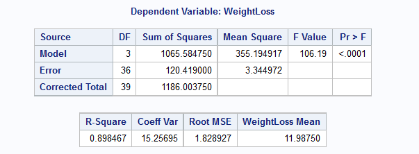
The f value is 106.19 and is associated with a significant p value. That is, a p value less than .05. While this tells us there is a significant association between diet type and weight loss, to understand that association we need to look at the output generated by the mean statement.

Here we show the finding graphically, as bar chart, with diet, the explanatory variable on the x-axis. And the mean weight loss, our response variable on the y axis. We see that the average one month weight loss for diet A is about 14.7 pounds. And that the average one month weight loss for diet B is about 9.3 pounds.

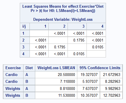
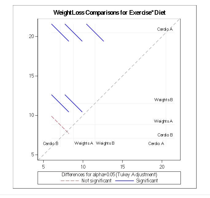
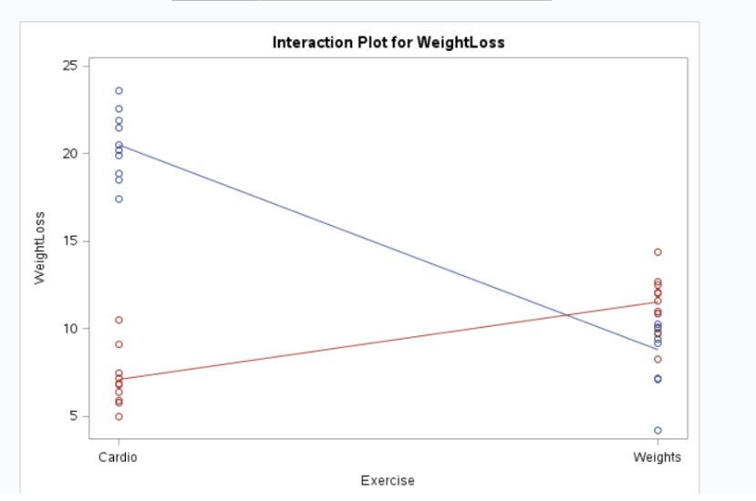
 Here, these results are shown graphically. As you can see, the relationship between diet and weight loss depends on which exercise program is being used. When using cardio, diet A is significantly better for weight loss than diet B. When using weights, diet B is significantly better for weight loss than diet A. Thus, we can say there’s a significant statistical interaction between the variables diet and weight loss. And the type of exercise, our third variable, moderates the association between diet and weigh loss.

 

A correlation coefficient assesses the degree of linear relationship between two variables. It ranges from +1 to -1. A correlation of +1 means that there is a perfect, positive, linear relationship between the two variables. A correlation of -1 means there is a perfect, negative linear relationship between the two variables. In both cases, knowing the value of one variable, you can perfectly predict the value of the second.

Below, you can find my code, (I used the Correlations task in SAS Studio) correlating two quantitative variables, the suicideper100th (suicide rate) variable with the alcconsumption (alcohol consumption) variable.

Please feel free to run it in SAS studio to make sure it works.

—————————————

/*
*
* Task code generated by SAS Studio 3.5
*
* Generated on ’19/1/17 – 3:51 μ.μ.’
* Generated by ‘epanagiotopoulo0’
* Generated on server ‘ODAWS02.ODA.SAS.COM’
* Generated on SAS platform ‘Linux LIN X64 3.10.0-514.2.2.el7.x86_64’
* Generated on SAS version ‘9.04.01M3P06242015’
* Generated on browser ‘Mozilla/5.0 (Windows NT 10.0; WOW64; rv:50.0) Gecko/20100101 Firefox/50.0’
* Generated on web client ‘https://odamid.oda.sas.com/SASStudio/main?locale=el_GR&zone=GMT%252B02%253A00&https%3A%2F%2Fodamid.oda.sas.com%2FSASStudio%2F=’
*
*/

ods noproctitle;
ods graphics / imagemap=on;

proc corr data=_TEMP1.GAPMINDER pearson nosimple noprob outp=WORK.Corr_stats
plots=matrix(histogram);
var suicideper100th;
with alcconsumption;
run;

—————————————

Let’s take a look at the scatter plot first.

From looking at the scatter plot, we can guess the association is positive. That is, a higher alcohol cunsumption rate is associated with higher suicide rate.

To locate the correlation coefficients of interest and the associated p values, we need to examine the Pearson Correlation Coefficient table here, and find the row and column where our two variables of interest intersect.

For the association between alcohol consumption rate and suicide rate, the correlation coefficient is approximately 0.35 with a p-value of 0.0001. This tells us that the relationship is statistically significant. Now we can actually interpret the scatter plots and the coefficients together.
The association between alcohol consumption rate and suicide rate is fairly strong and it’s also positive, as the scatter plot had already shown us, so it is statistically significant. That is, it’s highly unlikely that a relationship of this magnitude would be due to chance alone.

Post hoc tests are not necessary when conducting Pearson correlation. They are needed only when a research question includes a categorical explnatory variable with more than two levels. Because my explanatory variable and the context of correlation coeffeicient is quantitative, there’s no need to perform a post hoc test.

(A) Program syntax for chi-square test for SAHARA AFRICA

(B) program syntax for chi-square test of independence for MENA

results gotten were

(a) Sahara Africa

The chi-square prob for this test is 0.1052 which means that there are no enough evidence to reject null hypothesis. Since this is the case, i need not run a post hoc test.

(b) MENA initial chi-square result

Here, the chi-square prob is

(a) Comparison of lifeexpectancygroup 1 and 2 gave a chi-square prob of 0.1573 and indicates that this groups are statistically similar.

(b)

The chi-square prob from the comparison of group 1 and 3  above is 0.0113 which is less than the adjusted p-value for 3 comparison sets (0.05/3 = 0.0166). This show that group 1 and 3 are not similar.

(c)

The chi-square prob from the comparison of group 2 and 3 is 0.0003 as shown in (c). This shows that group 2 and 3 are also not similar.

A one-way analysis of variance (ANOVA) tests and provides graphs for differences among the means of a single categorical variable on a single continuous dependent variable. I used the One-Way ANOVA task in SAS Studio.

Step 1 –

Null hypothesis (N₀) = There is no association between the average life expectancy of a nations population and the urban rate of that nation.

Alternate hypothesis (N_A) = There is an association between the average life expectancy of a nations population and the urban rate of that nation.

Categorical explanatory variable = urban (multiple levels to this variable)

Quantitative response variable = lifeexpectancy

Program code:

/*
*
* Task code generated by SAS Studio 3.5
*
* Generated on ‘12/1/17 – 2:58 μ.μ.’
* Generated by ‘epanagiotopoulo0’
* Generated on server ‘ODAWS01.ODA.SAS.COM’
* Generated on SAS platform ‘Linux LIN X64 3.10.0-514.2.2.el7.x86_64’
* Generated on SAS version ‘9.04.01M3P06242015’
* Generated on browser ‘Mozilla/5.0 (Windows NT 10.0; WOW64; rv:50.0) Gecko/20100101 Firefox/50.0’
* Generated on web client ‘https://odamid.oda.sas.com/SASStudio/main?locale=el_GR&zone=GMT%252B02%253A00&https%3A%2F%2Fodamid.oda.sas.com%2FSASStudio%2F=’
*
*/

Title;
ods noproctitle;
ods graphics / imagemap=on;

proc glm data=_TEMP0.GAPMINDER;
class urbanrate;
model lifeexpectancy=urbanrate;
means urbanrate / duncan alpha=.05 hovtest=levene welch plots=none;
lsmeans urbanrate / alpha=.05;
run;
quit;

Program Results:

The results from the ANOVA F-test combined with the Duncan post hoc test show the alpha value equals 0.05 (5%). As this value is less than or equal to 0.05, we reject the null hypothesis. The results highlight that urban categories 3 (50% – 75% urban rates) and 4 (urban rate > 75%) are significantly different to categories 1 (1% – 25%) and 2 (25% – 50%). While categories 3 and 4 as well as 1 and 2 are not significantly different to each other.

Results Summary:

Following completion of an ANOVA F-Test with a Duncan post hoc test, the null hypothesis, that there is no association between the average life expectancy of a nation’s population and the urban rate of that nation, can be rejected. It is fair to assume that there is an association between the average life expectancy of a nation’s population and the urban rate of that nation. Urban rate categories 3 and 4 are significantly different to categories 1 and 2. The tests p value also falls within the acceptable standard to reject the null hypothesis (Alpha is less than or equal to 0.05).